Categories: Beginner
Hello,
First off, setting up Matplotlib on the BBBW (BeagleBone Black Wireless) will take forever. So, please stay patient and get all your dependencies.
…
So, first things firstly. We need to set up our BBBW image from
beagleboard.org/latest-images
and move on from that point forward.
…
Now, we need to set up our install for Matplotlib. We are going to need a set of lengthy-beefy tools/libraries.
Luckily, for the most part, kernel 4.19.x on the images have Python 3.6 and above or you can install it.
With the rest of those dependencies, you may need to do some research and look over how to install them, e.g. w/ pip3 or by way of you Linux package manager.
…
Now…hopefully we have accumulated the dependencies and we can move on.
Moving on thus far only requires us to stay patient while Matplotlib installs either via pip3 or your Distro package manager.
Here:
Okay…if you are using pip3 to install your Matplotlib distribution, okay. But, you can also install your Matplotlib distribution by means of your package manager like mentioned above.
See here:
Okay…wait forever for this install to take place. If it hangs, that is okay. It just takes a long, long, long time.
So, now that your install is finished without error, reboot.
Use these commands once your system on the BBBW reboots:
sudo apt update


sudo apt upgrade
Okay…
…
We are finally getting somewhere. We have our dependencies met, our Matplotlib install completed, and we can now pursue some nice visual effects for statistics.
See here:
from matplotlib import pyplot as plt, patches
import os
def main():
path = 'figures'
for i in range(21):
_fig, ax = plt.subplots()
x = range(3*i)
y = [n*n for n in x]
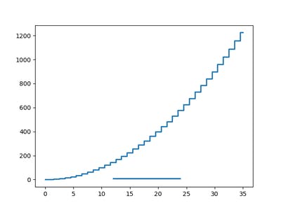
ax.add_patch(patches.Rectangle(xy=(i, 1), width=i, height=10))
plt.step(x, y, linewidth=2, where='mid')
figname = 'fig_{}.png'.format(i)
dest = os.path.join(path, figname)
plt.savefig(dest) # write image to file
plt.clf()
print('Done.')
main()
I found this source online at:
https://stackoverflow.com/questions/21884271/warning-about-too-many-open-figures.
I went here b/c I was suffering due to some error codes that prevented my system to run multiple (20) instances of the source being run under python3 <myfile.py>.
…
So, that source will basically run, end, and if you have created a directory named
figures,
21 files in.png format will be rendered for your viewing.
…
Try it out!
Oh and you can try other methods for writing photo files if necessary. There is a plethora of ideas online if you make the correct searches. There are many sites dedicated to statistics and Matplotlib too. Look here:
https://matplotlib.org/gallery/index.html
"there, a main page for examples!"
…
Seth
P.S. If you are having trouble and you do not know what to do to solve your equations, please do not hesitate to ask questions. Oh! Please use this software to transfer your files that write to the directories of your choice:
https://winscp.net/eng/index.php?#utm_source=winscp&utm_medium=app&utm_campaign=5.15.5.
Here is some source to play w/:
from mpl_toolkits import mplot3d

import numpy as np

from matplotlib import pyplot as plt, patches

import os


def main():

    path = "molt"

    _fig, ax = plt.subplots()

    for i in range(16):

        ax = plt.axes(projection="3d")

        zline = np.linspace(0, 15, 1000)

        xline = np.sin(zline)

        yline = np.cos(zline)

        ax.plot3D(xline, yline, zline, "red")

        zdata = 15 * np.random.random(100)

        xdata = np.sin(zdata) + 0.1 * np.random.randn(100)

        ydata = np.cos(zdata) + 0.1 * np.random.randn(100)

        ax.scatter3D(xdata, ydata, zdata, c=zdata, cmap="Greens")

        figname = "fig_{}.png".format(i)

        dest = os.path.join(path, figname)

        plt.savefig(dest)

        plt.cla()

    print("Completed!")


main()
You outcome should look like 17 photos in png. format and one is located below:
Comments are not currently available for this post.